Image Segmentation via Spectral Clustering

Abstract-Image Segmentation is a classic computer vision problem, which is also one of the foundation stones for many computer vision applications, e.g., 3D reconstruction, object tracking. This paper implemented two classic image segmentation methods via spectral clustering. Namely, the image segmentation based on K-means clustering and image segmentation based on normalized cuts and spectral clustering. Although nowadays most image segmentation methods are based on deep learning, the traditional solution can still be used in industrial environments, due to the computational cost. In this paper, we implemented two image segmentation methods using C++, and conduct testing on CIFAR-10 dataset. Solid experiments on the datasets demonstrate the robustness and effectiveness of the two implemented algorithms.

Introduction

Image segmentation is a computer vision task that involves dividing an image into meaningful and distinct regions or objects. It aims to partition an image into semantically cohesive regions based on similarities in color, texture, or other visual properties. It plays a crucial role in various applications, such as medical imaging, autonomous driving, object recognition, and scene understanding. By accurately delineating boundaries and identifying individual elements within an image, image segmentation enables advanced analysis, object tracking, and understanding of visual content. This process not only aids in extracting meaningful information from images but also paves the way for numerous downstream tasks and applications in diverse fields.

Related Works

As a classic computer vision task, the image segmentation problem has been widely studied during recent decades. Among all methods, the solutions can be categorized into two major aspects. Namely, traditional methods, and the deep learning-based methods. The former has received extensive attention in the early stage of image segmentation and requires fewer computing resources than methods based on deep learning, it is still widely used in scenes where the image background is simple but computing resources are limited. The latter is currently a research hotspot. With the increase in the complexity of the network model, the image segmentation effect is still on the rise.

Traditional Methods

These traditional approaches often rely on handcrafted features, such as color, texture, or edge information, combined with sophisticated algorithms. These methods can be categorized as thresholding methods, edge-based methods, region-based methods, Clustering-based methods. One commonly used technique is thresholding, where pixel intensities are compared to a fixed threshold value to distinguish between foreground and background regions [1][2]. The threshold methods include global Thresholding, which use one threshold for whole image, variable thresholding, where the threshold value T can vary over the image, and multiple thresholding. This method is simple and computationally efficient, but it struggles with images containing complex backgrounds or varying lighting conditions. Another approach is region-based segmentation, which groups pixels based on their similarity in color, texture, or other features [3][4]. Popular algorithms like K-means clustering and mean-shift segmentation fall under this category. Region-based methods offer good results when dealing with homogeneous regions, but they often struggle with accurately capturing object boundaries and handling overlapping regions. Clustering-based algorithms, such as graph cuts [5], leverage graph theory to model image segmentation as an optimization problem. These methods excel in capturing object boundaries and handling irregular shapes. However, they require prior knowledge or user interactions to define the initial seeds or cost functions, limiting their applicability in fully automated scenarios. Additionally, edge-based techniques, such as the Canny edge detector or active contours, focus on detecting and tracing object boundaries using edge information [6]. While these methods can achieve precise boundaries, they may struggle with noise, incomplete edges, or complex object shapes.

Deep Learning-based Methods

Nowadays most image segmentation solutions are based on deep learning, since it provides significantly better results than traditional methods. Long et al. introduced Fully Convolutional Networks (FCNs), a significant advancement in deep learning-based models for semantic image segmentation [7]. FCNs exclusively consist of convolutional layers, allowing them to generate segmentation maps that match the size of the input image. Chen et al. developed a semantic segmentation algorithm by combining Convolutional Neural Networks (CNNs) with fully connected Conditional Random Fields (CRFs) [8]. Their approach exhibited superior accuracy in localizing segment boundaries compared to previous methods. Schwing and Urtasun proposed a deep structured network that integrates CNNs and fully connected CRFs for semantic image segmentation [9]. Through joint training, their model achieved promising results on the challenging PASCAL VOC 2012 dataset. Badrinarayanan et al. presented SegNet, an architecture based on fully convolutional encoder-decoder networks for image segmentation [10]. SegNet’s segmentation engine comprises an encoder network, identical in topology to VGG16’s 13 convolutional layers, and a corresponding decoder network followed by a pixel-wise classification layer. Taking inspiration from the success of large models in natural language processing [11], researchers have also explored their application in image segmentation. Meta AI proposed the “Segment Anything” model, which is designed and trained to be promptable, enabling it to transfer knowledge to new image distributions and tasks.

Main Contributions

The main contribution of this paper is as follows:

• A C plus plus implementation of K-means clustering for color-based image segmentation is provided in this project.
• A C plus plus implementation of normalized-cut algorithm and spectral clustering image segmentation is provided in this project.
• Solid experiments based on our implemented solutions are conducted, and comparisons with each algorithm are presented.

The rest of the paper is organized as follows. Related works are presented in section II. Section III is the problem statement, the mathematical description of the problem is introduced. The details of the implemented two segmentation algorithms are in section IV, and experiments are conducted, and results are shown in section V, and in section VI we draw conclusions and future improvements.

Problem Statement

This paper focuses on images segmentation problem. Given $n$ unlabeled data points $ {x_1,x_2,\ldots,x_n} $ with $ x_i\in R^d $ and number of desired classes $K$ with no labels given this paper is trying to find cohesive clusters so that similar input data can be grouped. And the intra-class similarity is high, while the inter-class similarity is low.

Method

K-means Clustering

K-means is a popular clustering algorithm used in image segmentation. It aims to partition an image into distinct regions based on similarity of pixel values. K-means starts by randomly selecting $K$ initial cluster centers. Each pixel in the image is then assigned to the cluster with the closest center, based on the Euclidean distance between the pixel’s color values and the center’s color values. We use pseudo-random number generator based on Mersenne Twister [12] to generate $k$ color vectors from 0-255 in our implementation. After the initial assignment, the algorithm calculates the mean color values ${\mu_j\in R^3:1\le j\le K}$ for each cluster, based on the pixels assigned to it. These mean values become the new cluster centers.

$$
C_i=\arg{\min_{1\le j\le K}{d}}\left(x_i,\mu_j\right)
$$

$$
\mu_j=\frac{\sum_{i=1}^{n}{1{c_i=j}x_i}}{\sum_{i=1}^{n}{1{c_i=j}}}
$$

The assignment and recalculation steps are repeated iteratively until convergence, when the cluster centers no longer change significantly. Once convergence is reached, the image pixels are classified into K segments based on their final cluster assignments. Each segment represents a distinct region of similar pixel values. By varying the number of clusters K, the algorithm can produce different levels of segmentation granularity. To get better segmentation result, our method will perform k-means segmentation for one image multiple times with random generated initial values, and then find the best result among these segmentation result. Namely, find the best result corresponding to the minimum g, where $g=\sum_{i}|samples_i-centers_{labels_i}|^2$.

Normalized-cut algorithm

The normalized-cut algorithm considers the image as a graph and performs graph cut to segment images in to two clusters. Represent the image as a graph $G\left(V,E\right)$, where vertex $V$ represents each pixel in the image, and weighted edge $E$ represents the connectivity between pixels. Let two disjoint sets be $A, B$, where $A \cap B\ =V, A \cup B =\emptyset$. Then, the dissimilarity between the two pieces can be measured by calculating the combined weight of the removed edges. In graph theory, this measurement is referred to as the “cut”.

$$cut\left(A,B\right)=\sum_{u\in A,v\in B}\omega\left(u,v\right)$$

The image segmentation problem then can be transformed into finding the minimum cut of the graph. However, the minimum cut criteria will result in cutting small sets of isolated nodes in the graph, which are isolated pixels in the image. To avoid this issue, the Normalized cut introduced a novel metric for quantifying the disassociation between two groups. Instead of solely considering the total weight of edges connecting the partitions, they metric calculates the cut cost relative to the overall edge connections involving all nodes in the graph.

$$
Ncut\left(A,B\right)=\frac{cut\left(A,B\right)}{asso\left(A,V\right)}+\frac{cut\left(A,B\right)}{asso\left(B,V\right)}
$$

Where $asso\left(A,V\right)=\sum_{u\in A,t\in V}\omega\left(u,t\right)$ is the sum up connection from nodes in A to all nodes in the graph, and $asso\left(B,V\right)$ is defined similarly. Let x be an $N=\left|V\right|$ vector, and $x_i=1$ when $V_i\in A, x_i=-1 when V_i\in B$. $d\left(i\right)=\sum_{j}\omega\left(i,j\right)$ is the sum up connection from $V_i$ to other vertices. The $Ncut\left(A,B\right)$ can be rewritten as follows.

$$
Ncut(A, B)= \frac{\sum_{\left(\boldsymbol{x_i}>0, \boldsymbol{x_j}<0\right)}-w_{ij} \boldsymbol{x_i} \boldsymbol{x_j}}{\sum_{\boldsymbol{x_i}>0} \boldsymbol{d_i}}
+\frac{\sum_{\left(\boldsymbol{x_i}<0, \boldsymbol{x_j}>0\right)}-w_{ij} \boldsymbol{x_i} \boldsymbol{x_j}}{\sum_{\boldsymbol{x_i}<0} \boldsymbol{d_i}}
$$

Let D be an $N\times N$ diagonal matrix, W be an $N\times N$ symmetrical matrix with $W\left(i,j\right)=\omega_{ij}$. Then the $Ncut$ function can be rewritten as follows.

$$
Ncut\left(A,B\right)=\frac{\left(\boldsymbol{x}^T(\mathbf{D}-\mathbf{W}) \boldsymbol{x}+\mathbf{1}^T(\mathbf{D}-\mathbf{W}) \mathbf{1}\right)}{k(1-k) \mathbf{1}^T \mathbf{D} \mathbf{1}}+\frac{2(1-2 k) \mathbf{1}^T(\mathbf{D}-\mathbf{W}) \boldsymbol{x}}{k(1-k) \mathbf{1}^T \mathbf{D} \mathbf{1}}
$$

$$
=\frac{[(\mathbf{1}+\boldsymbol{x})-b(\mathbf{1}-\boldsymbol{x})]^T(\mathbf{D}-\mathbf{W})[(\mathbf{1}+\boldsymbol{x})-b(\mathbf{1}-\boldsymbol{x})]}{b \mathbf{1}^T \mathbf{D} \mathbf{1}}
$$

Where $b=\frac{k}{1-k}$, $k=\frac{\sum_{x_i>0}{\boldsymbol{d_i}}}{\sum_{i}{\boldsymbol{d_i}}}$
Then putting everything together, the minimum cut can be formulated as follows.

$$
\min \boldsymbol{x} N \operatorname{cut}(\boldsymbol{x})=\min y \frac{\boldsymbol{y}^T(\boldsymbol{D}-\boldsymbol{W}) \boldsymbol{y}}{\boldsymbol{y}^T \boldsymbol{D} \boldsymbol{y}}
$$

The normalized cut problem can be solved by calculating the second smallest eigenvector of the following equation.

$$
\left(\boldsymbol{D}-\boldsymbol{W}\right)\boldsymbol{y}=\lambda\boldsymbol{Dy}
$$

$$
\mathbf{D}^{-\frac{1}{2}}(\mathbf{D}-\mathbf{W}) \mathbf{D}^{-\frac{1}{2}} \boldsymbol{z}=\lambda \boldsymbol{z}
$$

Where $\boldsymbol{z}=\boldsymbol{D}^\frac{1}{2} \boldsymbol{y}$.
Finally, recursively calling the process for multiple partition.

Experiment

In the experimental section, this paper initially presents the implementation process of the algorithm and the selection of certain parameters. Subsequently, we provide a detailed comparison of the performance and shortcomings of the two algorithms.

System Setup

All algorithms in this paper are implemented in C++. The chosen data-set for testing is the CIFAR-10 data-set, which consists of 6000 images with a resolution of 32x32 pixels. This data-set is primarily used in the field of image classification, providing 10 class labels but no ground truth segmentation for the images. The data used in this paper is in binary format. Initially, the C++ standard library’s binary file I/O library is employed to read the binary data. Then, the data is segmented according to the format provided by the data-set, and the segmented data is stored in OpenCV Mats for further processing.

For the k-means segmentation algorithm, the initial cluster centers are generated using the Mersenne Twister-based pseudo-random number generator mt19937, which ensures good clustering results. To maximize the clustering effectiveness, the algorithm is iterated 100 times with different random initialization in 10 attempts. Experimental results have shown that this configuration yields stable results, minimizing the impact of random initialization and achieving optimal segmentation outcomes.

In the Normalized Cut algorithm for image segmentation, the definition of edge weights is as follows.

$$
w_{ij}= e^{\frac{-\left|F_{(i)}-F_{(j)}\right|_2^2}{\sigma_I^2}} *
$$

$$
\begin{cases}=e^{\frac{-\left|X_{(i)}-X_{(j)}\right|_2^2}{\sigma_X^2}} & \text { if }|X(i)-X(j)|_2<r \ , =0 & \text { otherwise. }\end{cases}
$$

where, $r$ represents the pixel neighborhood radius. The vector $F(i)$ is defined as
$[v, v * s * sin(h), v * s * cos(h)]^T$. Where h, s, and v are the three components of the image’s HSV color space. It is important to note that the HSV definition in OpenCV differs from the standard definition, requiring special handling. The vector X(i) represents the coordinates of the pixel. In this experiment, we set $\sigma_I = 0.01, \sigma_X = 4.0$, and $r = 5$. The color space conversion and computation of feature values in this implementation utilize functions provided by OpenCV.

Segmentation Experiment

This section will show the segmentation result for airplane, house, and deer images.

Figure 1: Airplane Segmentation Result
In the given airplane images shown in Figure.1, both algorithms achieved good classification results due to the simple background. However, the k-means-based algorithm, which clusters based solely on color, may result in splitting an airplane into multiple disconnected regions, affecting the segmentation outcome. On the other hand, the Normalized Cut method considers both distance and color in edge weights, leading to a more cohesive segmentation of the airplane and yielding better results.

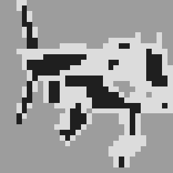
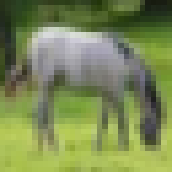
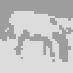
The segmentation results of the horse, as shown in Figure.2, demonstrate that both algorithms experience a certain degree of performance degradation as the complexity of the background increases.

Figure 2: Horse Segmentation Result
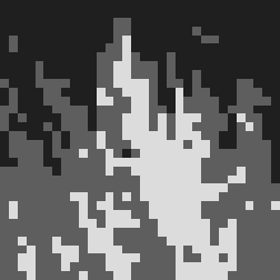
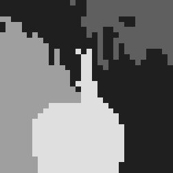
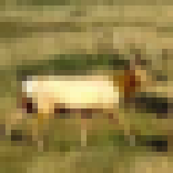
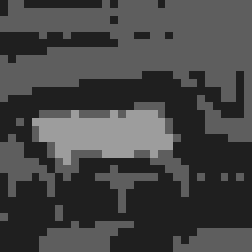
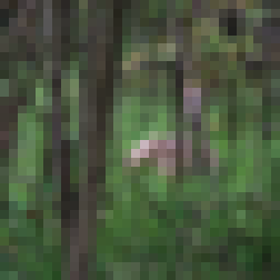
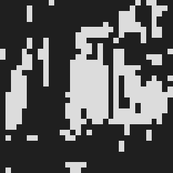
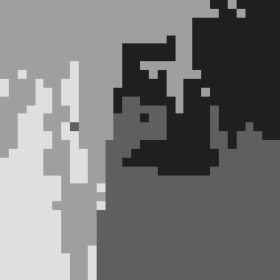
The segmentation results of the deer, as shown in figure.3, indicate that as the background complexity increases and includes multiple colors with significant differences, the performance of the k-means clustering model deteriorates significantly. On the other hand, the segmentation method based on Normalized Cut performs relatively well because it takes into account minimizing outliers during segmentation and incorporates both positional and color information in the edge weights. Figure 3: Deer Segmentation Result

Failure Analysis

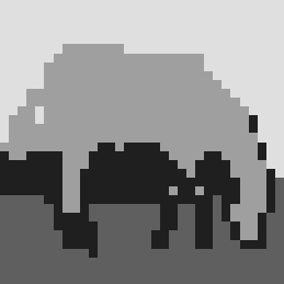
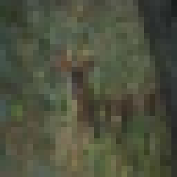
As the background complexity increases and the target region becomes less distinct, both classification algorithms struggle to achieve satisfactory results. The classification outcomes for complex backgrounds are displayed in Figure.4.

Figure 4: Segment failed images
The segmentation difficulty is high for the above images, and even for the human eye, it is challenging to distinguish them at low resolution. Both algorithms show poor segmentation performance, but Normalized Cut can significantly reduce the fragmentation of the segmentation.

Conclusion

In this work, we implemented two image segmentation approaches. First, we implemented an image segmentation algorithm based on K-means clustering, and we clustered using different color features, we mainly discuss the case of clustering into 4 categories. Secondly, this paper implements the algorithm based on Normalized-cut algorithm for clustering. We discuss the situation of using this algorithm to cluster into two categories at beginning. Then, by introducing recursive hierarchical clustering, we extend the clustering algorithm to multiple Class clustering, and discuss the case of clustering into 4 classes. Experiments show that the K-means algorithm has a better clustering effect in images with simple background and obvious color distribution, while the effect of Normalized-cut algorithm is more effective in images with uniform color distribution and no obvious distribution. However, for images with complex backgrounds, both types of segmentation algorithms perform poorly. Due to the lack of true values in this data set, it is difficult to do quantitative analysis on the clustering effect. In addition, this paper does not consider the sparse structure of the matrix when solving the eigenvalues, and still uses the general eigenvalue solving algorithm, the calculation performance has a certain loss. These issues still require further research in the future.

Reference

[1] Y.-J. Zhang, “An overview of image and video segmentation in the last 40 years,” Advances in Image and Video Segmentation, pp. 1–16, 2006.
[2] T. Lindeberg and M.-X. Li, “Segmentation and classification of edges using minimum description length approximation and complementary junction cues,” Computer Vision and Image Understanding, vol. 67, no. 1, pp. 88–98, 1997.
[3] M. R. Khokher, A. Ghafoor, and A. M. Siddiqui, “Image segmentation using multilevel graph cuts and graph development using fuzzy rule-based system,” IET image processing, vol. 7, no. 3, pp. 201–211, 2013.
[4] N. Senthilkumaran and R. Rajesh, “Image segmentation-a survey of soft computing approaches,” in 2009 International Conference on Advances in Recent Technologies in Communication and Computing. IEEE, 2009, pp. 844–846.
[5] J. Shi and J. Malik, “Normalized cuts and image segmentation,” in Proceedings of IEEE Computer Society Conference on Computer Vision and Pattern Recognition, Jun. 1997, pp. 731–737, iSSN: 1063-6919.
[6] S. S. Al-Amri, N. Kalyankar, and S. Khamitkar, “Image segmentation by using edge detection,” International journal on computer science and engineering, vol. 2, no. 3, pp. 804–807, 2010.
[7] J. Long, E. Shelhamer, and T. Darrell, “Fully convolutional networks for semantic segmentation,” in Proceedings of the IEEE conference on computer vision and pattern recognition, 2015, pp. 3431–3440.
[8] L.-C. Chen, G. Papandreou, I. Kokkinos, K. Murphy, and A. L. Yuille, “Semantic image segmentation with deep convolutional nets and fully connected crfs,” arXiv preprint arXiv:1412.7062, 2014.
[9] A. G. Schwing and R. Urtasun, “Fully connected deep structured networks,” arXiv preprint arXiv:1503.02351, 2015.
[10] V. Badrinarayanan, A. Kendall, and R. Cipolla, “Segnet: A deep convolutional encoder-decoder architecture for image segmentation,” IEEE transactions on pattern analysis and machine intelligence, vol. 39, no. 12, pp. 2481–2495, 2017.
[11] A. Kirillov, E. Mintun, N. Ravi, H. Mao, C. Rolland, L. Gustafson, T. Xiao, S. Whitehead, A. C. Berg, W.-Y. Lo, P. Dollár, and R. Girshick, “Segment anything,” 2023.
[12] M. Matsumoto and T. Nishimura, “Mersenne twister: A 623-dimensionally equidistributed uniform pseudo-random number generator,” ACM Trans. Model. Comput. Simul., vol. 8, no. 1, p. 3–30, jan 1998. [Online]. Available: https://doi.org/10.1145/272991.272995

Appendix

Source Code

The source code of this project is available at here.

PDF Version

The PDF version of this paper is available at here.

---

EOF