Simulation Setup
Isaac Gym provides a simulation interface that lets you create dynamic environments for training intelligent agents. The API is procedural and data-oriented rather than object-oriented. This facilitates efficient exchange of information between the core implementation written in C++ and client scripts written in Python. For example, rather than working with hierarchical collections of body and joint objects, Isaac Gym uses flat data arrays to represent the state and controls of the simulation. This makes it easy to work with the data using common Python libraries like NumPy, which provides efficient methods to manipulate multidimensional arrays. It is also possible to access the simulation data as CPU or GPU tensors that can be shared with common deep learning frameworks like PyTorch.
The core API, including supporting data types and constants, is defined in the gymapi module:
from isaacgym import gymapi
All of the Gym API functions can be accessed as methods of a singleton Gym object acquired on startup:
gym = gymapi.acquire_gym()
Creating a Simulation
The gym object by itself doesn’t do very much. It only serves as a proxy for the Gym API. To create a simulation, you need to call the create_sim method:
sim_params = gymapi.SimParams()
sim = gym.create_sim(compute_device_id, graphics_device_id, gymapi.SIM_PHYSX, sim_params)
The sim object contains physics and graphics contexts that will allow you to load assets, create environments, and interact with the simulation.
The first argument to create_sim is the compute device ordinal, which selects the GPU for physics simulation. The second argument is the graphics device ordinal, which selects the GPU for rendering. In multi-GPU systems, you can use different devices to perform these roles. For headless simulation (without a viewer) that doesn’t require any sensor rendering, you can set the graphics device to -1, and no graphics context will be created.
The third argument specifies which physics backend you wish to use. Presently, the choices are SIM_PHYSX or SIM_FLEX.
The PhysX backend offers robust rigid body and articulation simulation that can run on either CPU or GPU. It is presently the only backend that fully supports the new tensor API.
The Flex backend offers soft body and rigid body simulation that runs entirely on the GPU, but it does not fully support the tensor API yet.
The last argument to create_sim contains additional simulation parameters, discussed below.
Simulation Parameters
The simulation parameters allow you to configure the details of physics simulation. The settings may vary depending on the physics engine and the characteristics of the task to be simulated. Picking the right parameters is important for simulation stability and performance. The folling snippet shows examples of physics parameters:
# get default set of parameters
sim_params = gymapi.SimParams()

# set common parameters
sim_params.dt = 1 / 60
sim_params.substeps = 2
sim_params.up_axis = gymapi.UP_AXIS_Z
sim_params.gravity = gymapi.Vec3(0.0, 0.0, -9.8)

# set PhysX-specific parameters
sim_params.physx.use_gpu = True
sim_params.physx.solver_type = 1
sim_params.physx.num_position_iterations = 6
sim_params.physx.num_velocity_iterations = 1
sim_params.physx.contact_offset = 0.01
sim_params.physx.rest_offset = 0.0

# set Flex-specific parameters
sim_params.flex.solver_type = 5
sim_params.flex.num_outer_iterations = 4
sim_params.flex.num_inner_iterations = 20
sim_params.flex.relaxation = 0.8
sim_params.flex.warm_start = 0.5

# create sim with these parameters
sim = gym.create_sim(compute_device_id, graphics_device_id, physics_engine, sim_params)
Some of the parameters are independent of the physics engine, like simulation rate, up axis, or gravity. Others apply only to a specific physics engine (grouped under .physx and .flex). If the simulation is meant to run with only a specific physics engine, it is not necessary to specify the parameters for the other. Providing parameters for both engines will allow for easily selecting the engine at runtime, e.g. based on a command line argument.
For more information about simulation parameters, see:
Up Axis
Isaac Gym supports both y-up and z-up simulations. Although z-up is more common in robotics and research communities, Gym defaults to y-up for legacy reasons. This may change in the future, but in the meantime it is not hard to create a z-up simulation. The most important thing is to configure the up_axis and gravity in SimParams when creating the simulation:
sim_params.up_axis = gymapi.UP_AXIS_Z
sim_params.gravity = gymapi.Vec3(0.0, 0.0, -9.8)
Another place where the choice of z-up needs special attention is when creating the ground plane, discussed below.
Creating a Ground Plane
Most simulations need a ground plane, unless they take place in zero gravity. You can configure and create the ground plane like this:
# configure the ground plane
plane_params = gymapi.PlaneParams()
plane_params.normal = gymapi.Vec3(0, 0, 1) # z-up!
plane_params.distance = 0
plane_params.static_friction = 1
plane_params.dynamic_friction = 1
plane_params.restitution = 0

# create the ground plane
gym.add_ground(sim, plane_params)
The plane normal parameter defines the plane orientation and depends on the choice of up axis. Use (0, 0, 1) for z-up and (0, 1, 0) for y-up. It is possible to specify a normal vector that is not axis aligned to obtain a tilted ground plane.
The distance parameter defines the distance of the plane from the origin. The static_friction and dynamic_friction are the coefficients of static and dynamic friction. The restitution coefficient can be used to control the elasticity of collisions with the ground plane (amount of bounce).
Loading Assets
Gym currently supports loading URDF and MJCF file formats. Loading an asset file creates a GymAsset object that includes the definiton of all the bodies, collision shapes, visual attachments, joints, and degrees of freedom (DOFs). Soft bodies and particles are also supported with some formats.
When loading an asset, you specify the asset root directory and the asset path relative to the root. This split is necessary because the importers sometimes need to search for external reference files like meshes or materials within the asset directory tree. The asset root directory can be specified as an absolute path or as a path relative to the current working directory. In our Python examples, we load assets like this:
asset_root = "../../assets"
asset_file = "urdf/franka_description/robots/franka_panda.urdf"
asset = gym.load_asset(sim, asset_root, asset_file)
The load_asset method uses the file name extension to determine the asset file format. Supported extensions include .urdf for URDF files, and .xml for MJCF files.
Sometimes, you may wish to pass extra information to the asset importer. This is accomplished by specifying an optional AssetOptions parameter:
asset_options = gymapi.AssetOptions()
asset_options.fix_base_link = True
asset_options.armature = 0.01

asset = gym.load_asset(sim, asset_root, asset_file, asset_options)
The import options affect the physical and visual characteristics of the model, thus may have an impact on simulation stability and performance. More detail can be found in the chapter on Assets.
Loading an asset does not automatically add it to the simulation. A GymAsset serves as a blueprint for actors and can be instanced multiple times in a simulation with different poses and individualized properties.
Environments and Actors
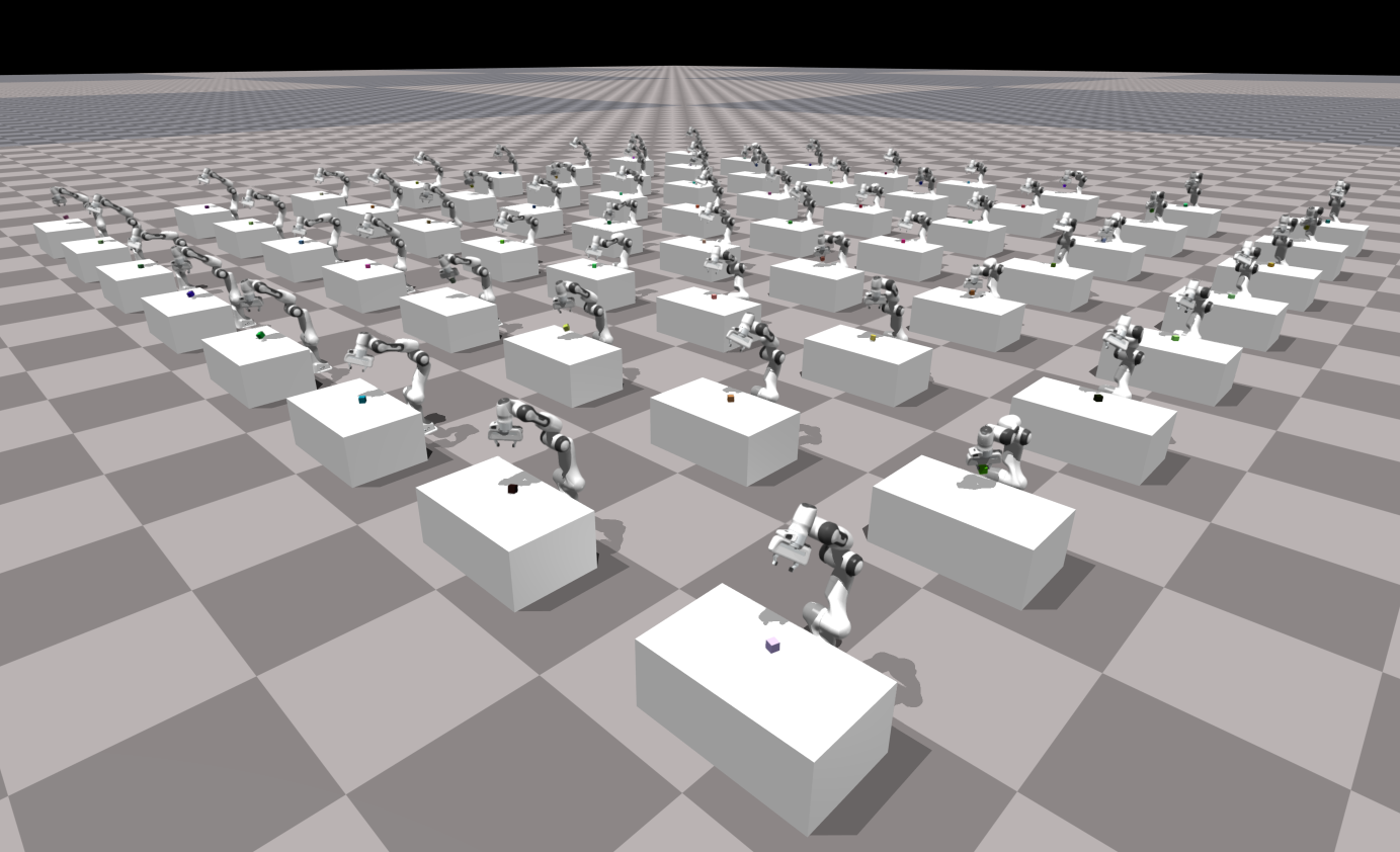
A snapshot from examples/franka_cube_ik.py with 64 environments simulated together on the GPU using PhysX. Each environment has three actors: a Franka arm, a table, and a box to be picked up. The environments are physically independent of each other, but are rendered together for easy monitoring. Getting the state of all envs and applying controls is done using a tensor-based API with PyTorch.
An environment consists of a collection of actors and sensors that are simulated together. Actors within an environment interact with each other physically. Their state is maintained by the physics engine and can be controlled using the control API discussed later. Sensors placed in an environment, like cameras, will be able to capture the actors in that environment.
An important design aspect of Isaac Gym is the ability to pack multiple instances of an environment into a single simulation. This is important in application areas like reinforcement learning, where a large number of runs is required to train agents to perform certain tasks. With Isaac Gym, you can run tens, hundreds, or even thousands of environment instances in lockstep. You can randomize the initial conditions in each environment, like layout, actor poses, and even the actors themselves. You can randomize the physical, visual, and control properties of all the actors.
There are several advantages to packing multiple environments into a single simulation, but the overall reason is performance. Many scenarios are actually quite simple. You might have a humanoid model learning to walk on a flat ground plane or an articulated robotic arm learning to pick up items in a cupboard. There is a certain amount of overhead involved in running each time step of a simulation. By packing multiple simple environments into a single simulation, we minimize that overhead and increase the overall computational density. This means that more time is spent on doing meaningful computations compared to the setup time required to launch the computations and gather the results.
Isaac Gym provides a simple procedural API for creating environments and populating them with actors. This is more useful than just loading static scenes from files, because it allows you to control the positioning and properties of all the actors as they are added to the scene. Before adding actors, you must create an environment:
spacing = 2.0
lower = gymapi.Vec3(-spacing, 0.0, -spacing)
upper = gymapi.Vec3(spacing, spacing, spacing)

env = gym.create_env(sim, lower, upper, 8)
Each env has its own coordinate space, which gets embedded in the global simulation space. When creating an environment, we specify the local extents of the environment, which depend on the desired spacing between environment instances. As new environments get added to the simulation, they will be arranged in a 2D grid one row at a time. The last argument to create_env states how many envs to pack per row.
An actor is simply an instance of a GymAsset. To add an actor to an environment, you must specify the source asset, desired pose, and a few other details:
pose = gymapi.Transform()
pose.p = gymapi.Vec3(0.0, 1.0, 0.0)
pose.r = gymapi.Quat(-0.707107, 0.0, 0.0, 0.707107)

actor_handle = gym.create_actor(env, asset, pose, "MyActor", 0, 1)
Each actor must be placed in an environment. You cannot have an actor that doesn’t belong to an environment. The actor pose is defined in env-local coordinates using position vector p and orientation quaternion r. In the snippet above, the orientation is specified by the quaternion (-0.707107, 0.0, 0.0, 0.707107). The Quat constructor takes the arguments in (x, y, z, w) order, so this quaternion represents a -90 degree rotation about the x-axis. Such a rotation is necessary when loading an asset that is defined using z-up convention into a simulation that uses y-up convention. Isaac Gym provides a convenience collection of math helpers, including quaternion utilities, so the quaternion could be defined in axis-angle form like this:
pose.r = gymapi.Quat.from_axis_angle(gymapi.Vec3(1, 0, 0), -0.5 * math.pi)
More information about the math utilities can be found in Math Utilities.
The create_actor arguments after the pose are optional. You can specify a name for your actor, which is “MyActor” in this case. This makes it possible to look up the actor by name later. If you wish to do this, make sure that you assign unique names to all your actors within the same environment. Because names are optional, Isaac Gym doesn’t enforce uniqueness. Instead of looking actors up by name, you can save the actor handle returned by create_actor. This handle uniquely identifies the actor in its environment and avoids the computational cost of searching for it later.
The two integers at the end of the argument list are collision_group and collision_filter. These values play an important role in the physics simulation of actors.
collision_group is an integer that identifies the collision group to which the actor’s bodies will be assigned. Two bodies will only collide with each other if they belong to the same collision group. It is common to have one collision group per environment, in which case the group id corresponds to the environment index. This prevents actors in different environments from interacting with each other physically. In certain cases, you may wish to set up more than one collision group per environment for more fine-grained control. The value -1 is used for a special collision group that collides with all other groups. This can be used to create “shared” objects that can physically interact with actors in all environments.
collision_filter is a bit mask that lets you filter out collision between bodies. Two bodies will not collide if their collision filters have a common bit set. This value can be used to filter out self-collisons in multi-body actors or prevent certain kinds of objects in a scene from interacting physically.
When setting up the simulation, you can initialize all the environments in a single loop:
# set up the env grid
num_envs = 64
envs_per_row = 8
env_spacing = 2.0
env_lower = gymapi.Vec3(-env_spacing, 0.0, -env_spacing)
env_upper = gymapi.Vec3(env_spacing, env_spacing, env_spacing)

# cache some common handles for later use
envs = []
actor_handles = []

# create and populate the environments
for i in range(num_envs):
    env = gym.create_env(sim, env_lower, env_upper, envs_per_row)
    envs.append(env)

    height = random.uniform(1.0, 2.5)

    pose = gymapi.Transform()
    pose.p = gymapi.Vec3(0.0, height, 0.0)

    actor_handle = gym.create_actor(env, asset, pose, "MyActor", i, 1)
    actor_handles.append(actor_handle)
In the snippet above, all envs contain the same type of actor, but the actors spawn at a randomized height. Note that the collision group assigned to each actor corresponds to the environment index, which means that the actors from different environments will not interact with each other physically. As we construct the environments, we also cache some useful information in lists that can be easily accessed in subsequent code.
Presently, the procedural API for setting up the environments has some limitations. It is assumed that all environments are created and populated in sequence. You create an environment and add all the actors to it, then create another environment and add all its actors to it, and so on. Once you finish populating one environment and start populating the next one, you can no longer add actors to the previous environment. This has to do with how the data is organized internally to facilitate an efficient batch indexing scheme for the state cache. This restriction may be lifted in the future, but for now be aware of the limitations. This implies that you cannot add or remove actors in an environment after you finish setting it up. There are ways to “fake” having a dynamic number of actors in an environment, which will be discussed in another section.
Running the Simulation
After setting up the environment grid and other parameters, you can begin simulating. This is typically done in a loop where each iteration of the loop corresponds to one time step:
while True:
    # step the physics
    gym.simulate(sim)
    gym.fetch_results(sim, True)
Isaac Gym offers a variety of ways to query the state of the world and apply controls. You can also gather sensor snapshots and connect with external learning frameworks. These topics will be discussed in subsequent chapters.
Adding a Viewer
By default, the simulation does not create any visual feedback window. This allows the simulations to run on headless workstations or clusters with no monitors attached. When developing and testing, however, it is useful to be able to visualize the simulation. Isaac Gym comes with a simple integrated viewer that lets you see what’s going on in the simulation.
You create a viewer like this:
cam_props = gymapi.CameraProperties()
viewer = gym.create_viewer(sim, cam_props)
This pops up a window with the default dimensions. You can set different dimensions by customizing the isaacgym.gymapi.CameraProperties.
In order to update the viewer, you can execute this code during every iteration of the simulation loop:
gym.step_graphics(sim);
gym.draw_viewer(viewer, sim, True)
The step_graphics method synchronizes the visual representation of the simulation with the physics state. The draw_viewer method renders the latest snapshot in the viewer. They are separate methods, because step_graphics can be used even in the absence of a viewer, like when rendering camera sensors.
With this code, the viewer window will refresh as quickly as possible. For simple simulations, this will often be faster than real time, because each dt increment will be processed faster than that amount of real time elapses. To synchronize the visual update frequency with real time, you can add this statement at the end of your loop iteration:
gym.sync_frame_time(sim)
This will throttle down the simulation rate to real time. If the simulation is running slower than real time, this statement will have no effect.
If you wish to terminate the simulation when the viewer window is closed, you can condition your loop on the query_viewer_has_closed method, which will return True after the user closes the window.
A basic simulation loop that incorporates the viewer looks like this:
while not gym.query_viewer_has_closed(viewer):

    # step the physics
    gym.simulate(sim)
    gym.fetch_results(sim, True)

    # update the viewer
    gym.step_graphics(sim);
    gym.draw_viewer(viewer, sim, True)

    # Wait for dt to elapse in real time.
    # This synchronizes the physics simulation with the rendering rate.
    gym.sync_frame_time(sim)
Fullscreen mode for the viewer can be toggled with F11 when the viewer is in focus.
The Viewer GUI
When a viewer is created, a simple graphical user interface will be shown on the left side of the screen. Display of the GUI can be toggled on and off with the ‘Tab’ key.
The GUI has 4 separate tabs: Actors, Sim, Viewer, and Perf.
The Actors tab provides the ability to select an environment and an actor within that environment. There are three separate sub-tabs for the currently selected actor.
The Bodies sub-tab gives information about the active actor’s rigid bodies. It also allows for changing the display color of the actor bodies and toggling the visualization of the body axes.
The DOFs sub-tab displays information about the active actor’s degrees-of-freedom. The DOF properties are editable using the user interface, put please note that this is an experimental feature.
The Pose Override sub-tab can be used to manually set the actor’s pose using its degrees of freedom. This feature, when enabled, overrides the pose and drive targets of the selected actor with values set in the user interface using sliders. It can be a useful utility for interactively exploring or manipulating the degrees of freedom of an actor.
The Sim tab shows the physics simulation parameters. The parameters vary by simulation type (PhysX or Flex) and can be modified by the user.
The Viewer tab allows customizing common visualization options. A noteworthy feature is the ability to toggle between viewing the graphical representation of bodies and the physical shapes that are used by the physics engine. This can be helpful when debugging physics behavior.
The Perf tab shows internally measured performance of gym. The top slider, “Performance Measurement Window” specifies a number of frames over which performance is measured. The frame rate reports the average frames per second (FPS) over the previous measurement window. The rest of the performance measures are reported as an average value per frame over the specified number of frames.
Frame Time is the total time from when one step begins to when the next step begins
Physics simulation time is the time the physics solver is running.
Physics Data Copy is the amount of time spent copying simulation results.
Idle time is time spent idling, usually within
gym.sync_frame_time(sim).Viewer Rendering Time is the time spent rendering and displaying the viewer
Sensor Image Copy time is the time spent copying sensor image data from the GPU to the CPU.
Sensor Image Rendering time is the time spent rendering camera sensors, not including viewer camera, into GPU buffers.
Custom Mouse/Keyboard Input
To get mouse/keyboard input from the viewer, action events can be subscribed to and queried. For an example of how to do this, look at examples/projectiles.py:
gym.subscribe_viewer_keyboard_event(viewer, gymapi.KEY_SPACE, "space_shoot")
gym.subscribe_viewer_keyboard_event(viewer, gymapi.KEY_R, "reset")
gym.subscribe_viewer_mouse_event(viewer, gymapi.MOUSE_LEFT_BUTTON, "mouse_shoot")
...
while not gym.query_viewer_has_closed(viewer):
    ...
    for evt in gym.query_viewer_action_events(viewer):
        ...
Cleanup
At exit, the sim and viewer objects should be released as follows:
gym.destroy_viewer(viewer)
gym.destroy_sim(sim)